[Algorithm] How a chess engine works
Graph - how does chess look like in computer memory
Computer thinks of chess as states, each state is a board where pieces are placed. Each move changes from one state to another, constructs a graph. From one state, players may have plenty ways to make a move, expands the graph to many branches. That being said, what computer is going to deal with, is a tree in which each node is a state and each edge is a move. We call that a game tree - a directed graph that describes all possible game states. To give an illustration, let’s take a look at another board game which is much simpler but shares the same idea with chess: tic-tac-toe.

As in the above graph, from the initial state (depth = 0), the first player has 3 ways to make move, each move produces another state. From one among 3 states (depth = 1), the second player has another 5 ways to make move, expands the game-tree, and so on.
You’re may curious when the graph expansion stops? Well, it will stop itself either when one player wins the game, or the board is full, or it reaches the depth-level you want it to be, whatever comes first.
The game-tree on chess game is pretty similar, things that make chess harder are board size and pieces variety, which make the game-tree to have a lot of branches.
The actual algorithm
By now we have had an idea how the game can be represented in computer memory. But how computer makes decision? More specifically, how computer knows what is the right move to make?
Chess, along with tic-tac-toe, gomoku, reversi and many other board games are zero-sum games - the games in which players make move rotationally. One’s gain and other’s loss are exactly balanced and they will sum to 0 (zero-sum). Furthermore, they are also perfect-information games - where all game information, including game states, prices, qualities etc are perfectly known by both players.
There is a decision scheme (or decision algorithm) for that kind of game called minimax, allows computer to make decision by maximizing the minimum gain, or in other words, minimizing loss in the worst case. Easy enough? Let’s jump into the code:
func DoMiniMax(state State, depth int, computer int) int {
	if depth == 0 {
		return Eval(state)
	}

	moves, _ := state.PossibleMoves(computer)
	if computer == true {
		//maximizing player
		max := WORST
		for _, move := range moves {
			clone := state.Move(move)
			max = DoMiniMax(clone, depth-1, false)
		}
		return max
	} else {
		//minimizing player
		min := BEST
		for _, move := range moves {
			clone := state.Move(move)
			max = DoMiniMax(clone, depth-1, true)
		}
		return min;
	}
	return 0
}
Notice that the algorithm uses recursive function to expand the game tree. From one state, it expands the tree by searching for all possible moves, creates new state for each move, and then calls itself recursively on each new state.
Let’s analyze the algorithm a little bit to see how complicated it is: There are 2 components that introduce the time complexity, the for loop and the recursive call (assume that the Eval() function and the PossibleMoves() function cost nearly zero).
where \(m\) is number of possible moves at a particular state and \(d\) is the depth of that state
Now assume that all states have the same number of possible moves of \(m\), by induction:
\[\begin{align} T(d) & = m + m^2 + m^2T(d - 2)\\ & = m + m^2 + \cdots + m^{d}T(0)\\ & = \displaystyle\sum_{i=1}^{d} m^i \end{align}\]So the time complexity of above function is \(O(m^d)\) in which \(d\) is the depth and \(m\) is the number of possible moves in a state of that depth (assume that all states have the same number of possible moves). That’s considered extra-high complexity.
Optimizations
You might have realized the above algorithm is nothing but a simple brute-force algorithm. To be honest, it is. But nevertheless, we can do better than that by adding some optimizations
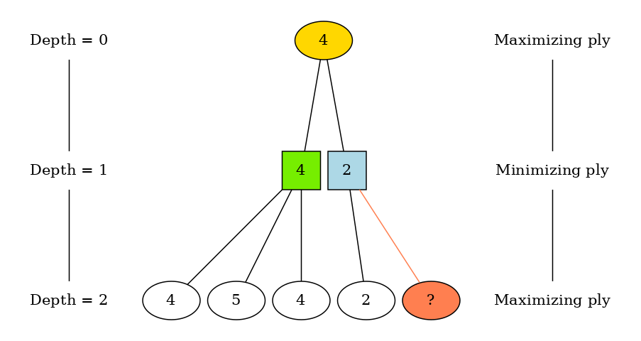
Take a look at the above graph, on the green branch, computer chose the smallest among 3 evaluated values [4, 5, 4] to determine the worst possible value of maximizing player. On the light-blue branch, the first value is calculated and equal to 2 thus the value of this branch should never be greater than 2. But since the value of green branch is 4, which is greater than the smallest value of the blue branch, the final value (golden node) will be 4 without being influenced by the coral node. That means the computer doesn’t need to evaluate this node.
The name of the above clever scheme is alpha-beta pruning algorithm. The algorithm is implemented by maintaining two values: alpha and beta which represent the minimum value that the maximizing player is assured, and the minimum value that the minimizing player is assured, respectively. Due to some cut-offs on branches, this scheme allows minimax to search deeper within the same amount of time as normal minimax. The search can go twice as deep with the same amount of computation, compared to the normal minimax. And the time complexity decreases from \(O(m^d)\) to \(O(\sqrt{m^d})\) in the best case - pretty impressive.
Now let’s see how it could be implemented in the code:
func DoMiniMax(state State, depth int, computer bool, alpha int, beta int) int {
	if depth == 0 {
		return Eval(state)
	}

	moves, _ := state.PossibleMoves(computer)
	if computer == true {
		//maximizing player
		max := WORST
		for _, move := range moves {
			clone := state.Move(move)
			max = DoMiniMax(clone, depth-1, false, alpha, beta)
            		alpha = MaxOf(alpha, max)

            		if alpha >= beta {
                		break
            		}
		}
		return max
	} else {
		//minimizing player
		min := BEST
		for _, move := range moves {
			clone := state.Move(move)
			min = DoMiniMax(clone, depth-1, true, alpha, beta)
            		beta = MinOf(beta, min)

            		if alpha >= beta {
                		break
            		}
		}
		return min;
	}
	return 0
}
As you can see in the above code snippet, the recursive function accepts two more variables as arguments: the alpha and beta values. For each child in the current states, it compares alpha with beta. When alpha is greater or equal to beta, which means other children do not affect the result, it calls break to drop all calculations on the other child branches.
Conclusion
Computer thinks of chess as a directed-graph that describes game states. Computer solves it by expanding and searching through the states to find the best move for it. It’s a brute-force algorithm but we can cut-off some unneeded branches to speed it up. In the next post, I will implement another vital part of the algorithm: the evaluation function.